How to hide the summary rows when combining Excel books with Power Query

In this article, I will show you how to hide only the summary row after joining multiple Excel books with summary rows in a power query.
If you have not read the following article, please read it first.

How to combine multiple excel books into one using Power Query and split it again using VBA
If you are sick and tired of wasting time with cut-and-paste to merge or split excel data, this article is for you.
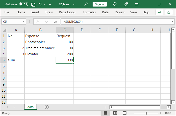
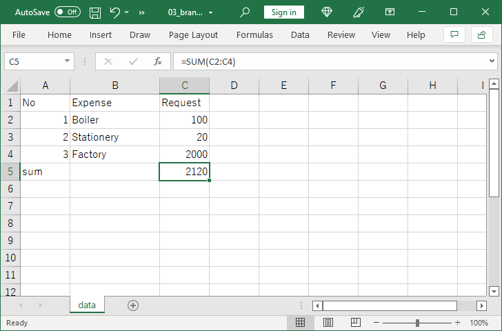
Data for the tutorial
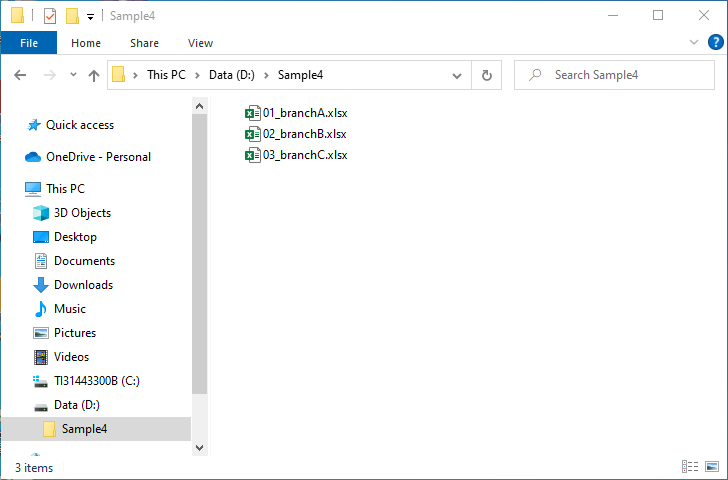
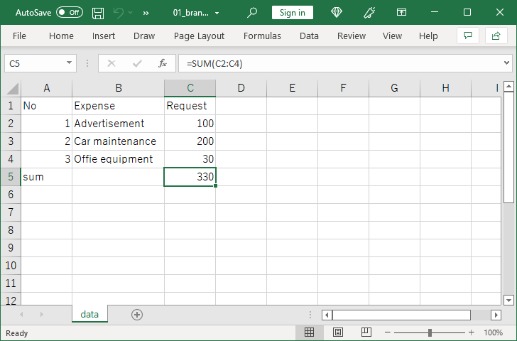
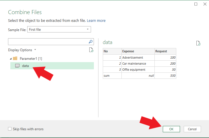
The figure shows the contents of "01_branchA.xlsx."
Tutorial to combine Excel books
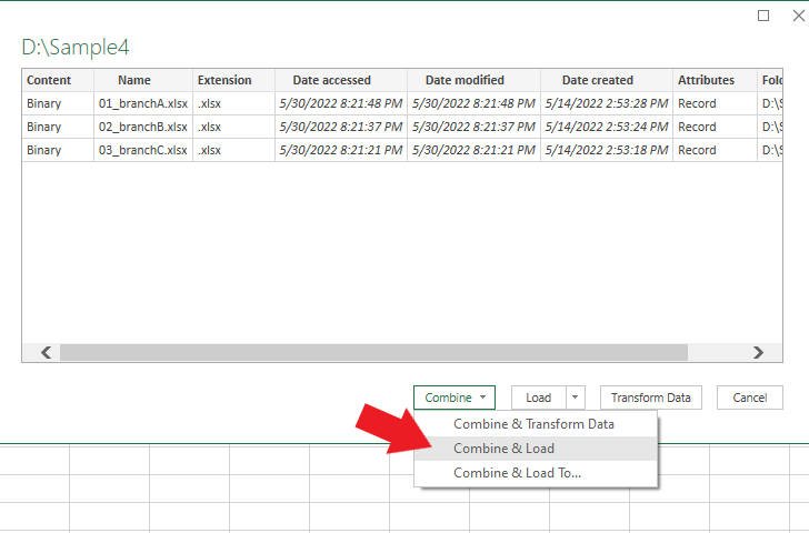
The combining method is the same as in the previous article, but I write it again here.
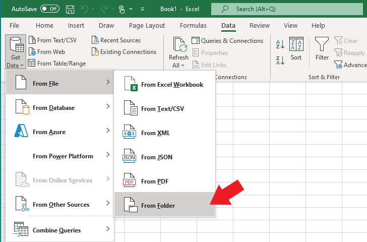
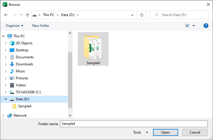
Then click “From File” and “From Folder.”
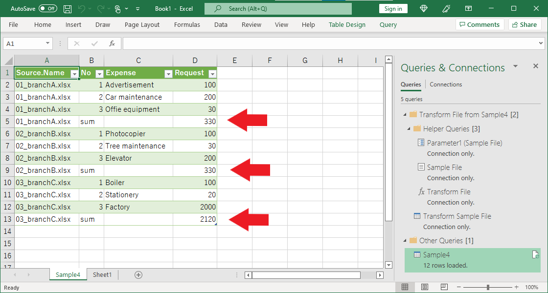
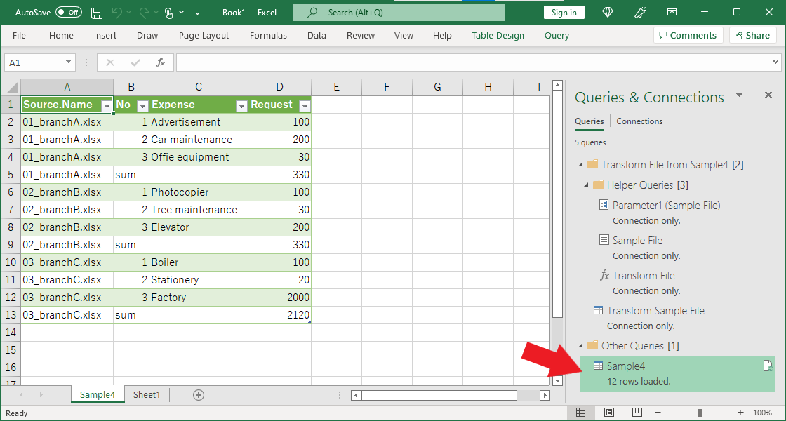
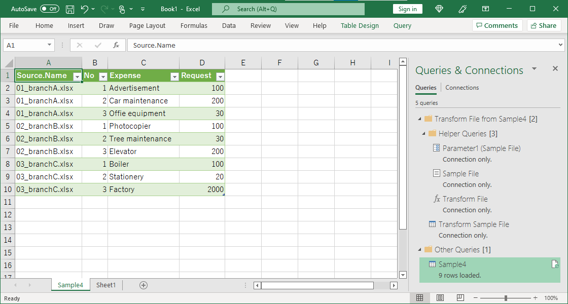
When the process is completed, the summary row of each Excel book will be imported as shown in the figure.
Tutorial to hide summary rows
This section describes how to prevent aggregate rows from appearing in the result of combining.
First, double-click “test4” in the “Queries & Connections” panel.
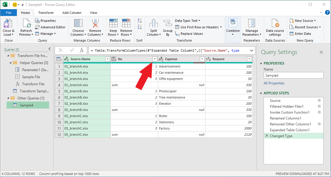
When the Power Query Editor launches, click the pull-down button in the second column for “No.”
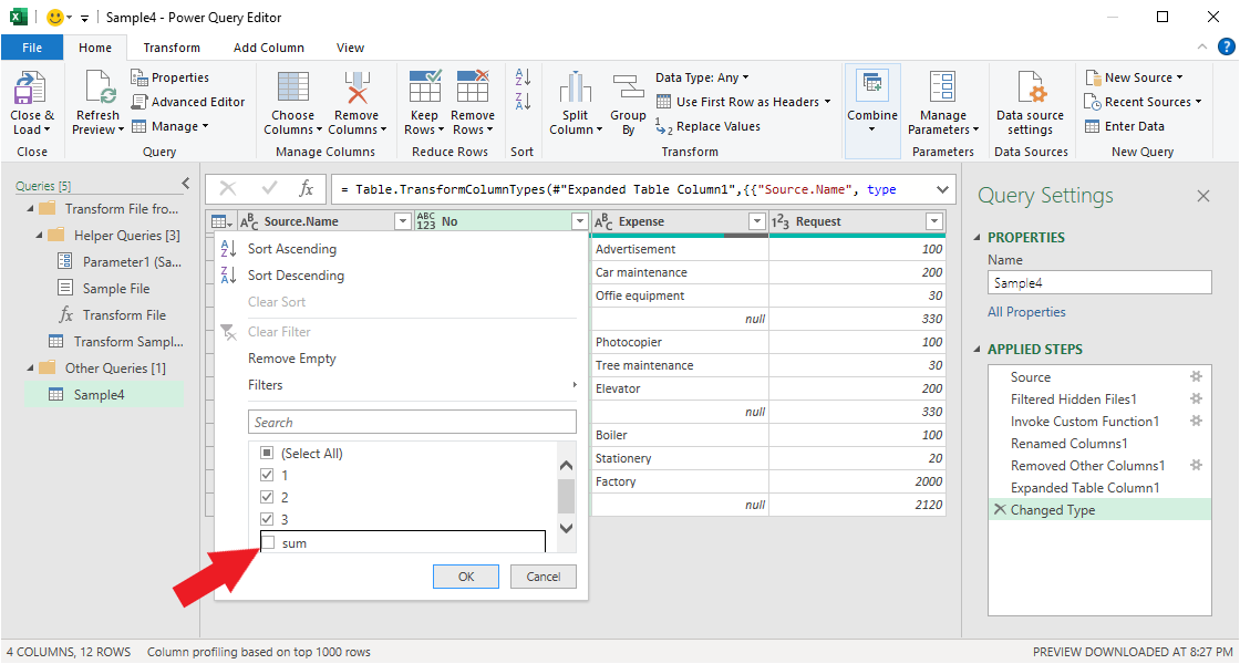
Uncheck “sum” and click the OK button.
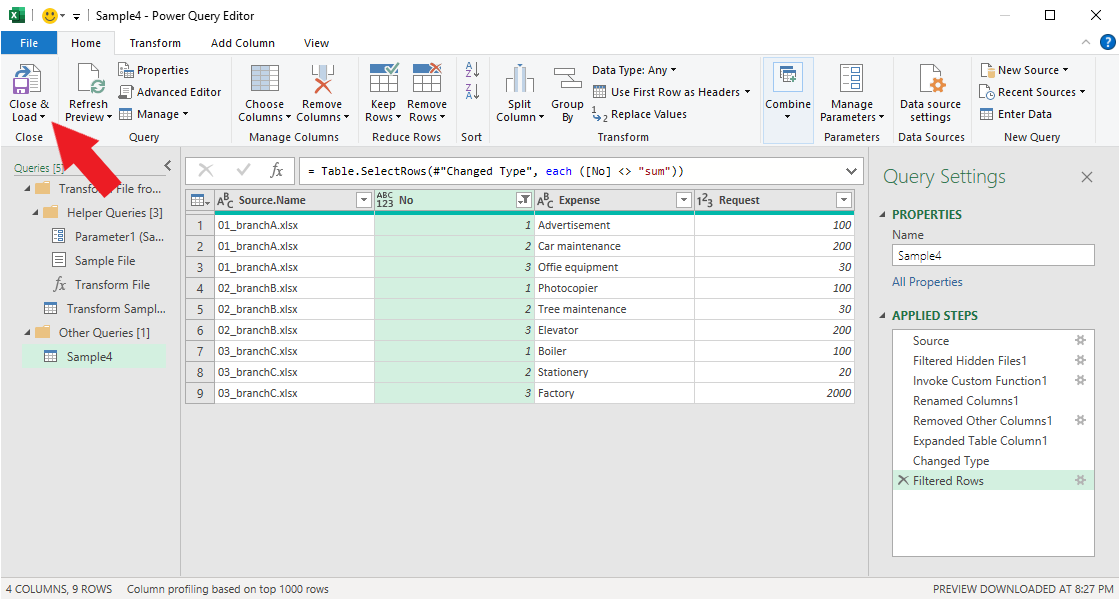
Click “Close & Load” in the upper left corner of the screen.
Completed. Summary rows are now hidden.